Introduction to diffusion and flow models for molecule structure prediction and molecule generations - I. flow and diffusion.

Preface

I recently had the privilege to be guided through a reading list of diffusion models on biomolecules’ structure prediction and generation by Hannes Stark from MIT CSAIL. In this post, I will document what I have learned and, hopefully, this post can serve as an educational resource for others interested in these topics.

I shall keep my language as concise as possible, yet aspiring readers can directly find the list at the end of the post and read ahead.

For reading time reason, this post will only contain information on flow and diffusion models. To find more on diffusion and flow models for molecule structure prediction and molecule generations, see my other posts. I also include some sample codes here.

Motivation

In machine learning when we talk about a parametric model, we want the parameters to compose a function that fits to our purpose. The function can be any function, by the universal approximation theorem, so naturally a probability density function can also be learned.

Given samples from a distribution, a natural question is: what does the distribution look like? Or more rigorously, what is the distribution in terms of its probability density function? By learning this distribution, we can either sample from it to generate unseen samples (generative modeling), or do various other things.

In variational inference, we want to evolve a simple distribution p, such as a vanilla gaussian, to approximate q, the supposedly complicated ground truth probability density. Usually this approximation is very mathy and relies heavily on assumptions, but one now can use a learned parametric model \(f_\theta\) to define q, either explicitly or implicitly.

Note: The paragraph above can be a bit hard to grasp, but imagine you have a play-doh at hand. At first, it is some simple shape, such as a sphere, and we pinch, punch, squeeze, finally putting it into more complicated forms, such as a car. The sphere in this example is p in the language of variational inference, the car is q, and the process of pinching, punching, and squeezing, is the model we learn.

Flow Models

Flow models do exactly what we described above. Probability distributions in general are measures with unit volume, and the process of morphing distributions can be seen as moving the volumes around such that the final output matches our goal. This move-around is what we call a flow. In flow models, we would like to learn how the distributions evolve over time.

Normailzing Flow

There were two main methods. One is called normalizing flow, where we model a sequence of invertible functions that sends p into q.¹ One problem with this approach is that each layer of the model encodes one map; therefore the effectiveness of the model depends heavily on how well each layer can capture the flow maps and the number of the flow maps. In general, normalizing flow performs well, but the error margin could be large if the model is not deep enough.

Continuous Normailzing Flow

The other approach generalizes over normalizing flow into a continuous setting.² People realize that the flow map is indeed implicitly determined by a vector field, and normalizing flow with k layers can been seen as taking k steps in the vector field using Euler method. The discretiztion can induce unwanted error, so why not simply learn the field and use a more accurate ODE solver to get the map? Neural ODE does exactly this by proposing an adjoint method that people can use to backpropagate the loss through the ODE solver without worrying about storing the intermediate steps within the solver. Because it can been seen as a continous case of normalizing flow, people call it continous normalizing flow, or simply CNF in most related papers.

A more mathematical description of CNF follows. We wish to construct a time‑dependent diffeomorphic (bijective, and whose inverse is differentiable) map, \(\phi : [0,1]\times \mathbb{R}^d \to \mathbb{R}^d\) with:

\[\frac{d}{dt}\,\phi_t(x) = v_t\bigl(\phi_t(x)\bigr) \tag{1}\] \[\phi_0(x) = x \tag{2}\]

Condtional Normailzing Flow

With the flow models, people can now learn to transform a simple distribution into a complicated one. Here is only but one problem: what would be the learning loss? You see, for continuous normalizing flow, since we are learning the vector field, in general we wish to minimize over

\[\mathcal{L}_{\mathrm{FM}}(\theta) = \mathbb{E}_{t,\,p_t(x)} \big\|v_t(x) - u_t(x)\big\|^2 \tag{3}\]

The loss here is natural, yet very hard to compute, as in fact we do not know exactly what \(u_t(x)\) is at any given moment. In fact, there are many of the possible ways to perform the flow. Take this visualization: Imagine you are sending your kid to school. Each morning, you are not gauranteed to take the same route, or even if you do, your velocity at a given moment can be different. Nonetheless, you can still put your kid in school before class.

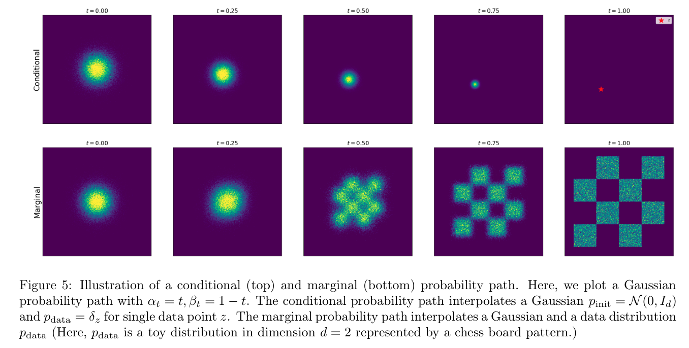
One solution is given by ³, where the authors propose to use a conditional loss

\[\mathcal{L}_{\mathrm{CFM}}(\theta) = \mathbb{E}_{t,\,q(x_{1}),\,p_t(x\mid x_{1})} \bigl\lVert v_{t}(x) - u_{t}(x \mid x_{1})\bigr\rVert^{2} \tag{4}\]

Here, \(u_{t}(x \mid x_{1})\) is the vector field conditioned on one sample selection \(x_{1}\) from the ground truth distribution q. What does this mean is that we randomly sample one point from the distribution q, and then treat the q as if it is the Dirac defined on that point or as if it is the gaussian centered around that point with minimal spread. Then we learn the conditional field \(u_{t}(x \mid x_{1})\) that produce \(p_{t}(x \mid x_{1})\), which is the probability density at time t, but conditioned on \(x_{1}\). See the figure below.

One good thing about conditional normalizing flow loss is that it shares the same minimizer with the conditional flow. Or in math terms,

\[\mathcal{L}_{FM}(\theta) \;=\; \mathcal{L}_{CFM}(\theta) \;+\; C, \tag{5}\]

where (C) is independent of (\theta). Their gradients coincide:

\[\nabla_\theta \mathcal{L}_{FM}(\theta) \;=\; \nabla_\theta \mathcal{L}_{CFM}(\theta). \tag{6}\]

Thus, they have the same minimizer \(\theta^{*}\). A proof of this can be found in ^{3 4 5}.

Diffusion, Markov Chain and Probability Path

“Creating noise from data is easy; creating data from noise is generative modeling.”⁶

Diffusion in a Nut Shell

The diffusion models draw inspirations from stochastic differential equations (SDE) in polluting the data with noise, and recover it by denoising.

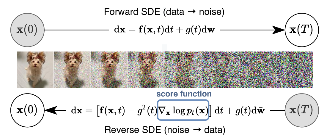
The figure above explains the diffusion process very well. During training time, we sample from the data distribution, pollute each of them by adding noises, and arrive at something that is completely noisy. The model in this process will try to capture the noise level at each given time t, and predict for us a denoising path. Then, during inference time, we use the learned model to learn a denoising path via which we can reconstruct a meaningful data point, such as a photo or a protein structure. The path we follow is defined by a function called score.

The key here in studying score-based diffusion is to understand the score function. It assumes the form \(\nabla_{\mathbf{x}} \log p_t(\mathbf{x})\). It is the gradient of some log likelihood, and as in the above figure, in the reverse denoising SDE, we would like to take a step against this gradient. However, notice here the term \(dt\) is an infinitesimal negative timestep. If we make it positive, that is, reparameterize it with a different variable, \(s = T - t\), the SDE becomes

\[\mathrm{d}x = \bigl[f(x,\,T - s) \;-\; g(T - s)^2\,\nabla_x\log p_{T - s}(x)\bigr]\,(-\mathrm{d}s) \;+\; g(T - s)\,\mathrm{d}\widetilde w_s, \tag{7}\]

which simplifies to:

\[\mathrm{d}x = \Bigl[-\,f(x,\,T - s) \;+\; g(T - s)^2\,\nabla_x\log p_{T - s}(x)\Bigr]\mathrm{d}s \;+\; g(T - s)\,\mathrm{d}\widetilde w_s. \tag{8}\]

For readers who have had previous experience in machine learning losses, it is very familiar if we ignore the stochastic terms, since minimizing the negative log likelihood (taking a step against this gradient) is equivalent to maximizing the likelihood \(p_t(\mathbf{x})\). In other words, in reverse diffusion process, we are simply maximizing the likelihood of having this data point at this time, \(p_t(\mathbf{x})\). For the attentive readers who are familiar with exponential classes of probability, or with the Boltzmann distribution, this gradient ascent in likelihood also translates into gradient descent in energy:

\[p(\mathbf{x}) \;=\; \frac{1}{Z}\,\exp\!\Bigl(-\tfrac{E(\mathbf{x})}{T}\Bigr), \tag{9}\]

Above is the probability density function of Boltzmann distribution. Put it into gradients:

\[\begin{aligned} \nabla_{\mathbf{x}}\,p(\mathbf{x}) &= \nabla_{\mathbf{x}}\!\Bigl[\tfrac{1}{Z}\,e^{-E(\mathbf{x})/T}\Bigr] \\ &= \frac{1}{Z}\,e^{-E(\mathbf{x})/T}\,\bigl(-\tfrac{1}{T}\bigr)\,\nabla_{\mathbf{x}}E(\mathbf{x}) \\ &= -\frac{1}{T}\,p(\mathbf{x})\,\nabla_{\mathbf{x}}E(\mathbf{x}). \end{aligned} \tag{10}\]

Here \(Z\) is treated conveniently as a constant. Thus,

\[\nabla_{\mathbf{x}}\,p(\mathbf{x}) \;\propto\; -\nabla_{\mathbf{x}}E(\mathbf{x}), \tag{11}\]

Now that we get the big picture, we can draw connections from diffusion to flow models. During inference, a diffusion model is only different to a flow model in that the deterministic process of flowing become stochastic. Apart from the step in the direction of a vector field, we add a random walk, or more precisely, a Brownian motion. On a high level, diffusion models trade off some qualtity in flow models’ generation to diversity, due to its stochastic nature.

Markov Chain

A markov chain or a markov process in statistics is a stochatic process describing a sequence of events, in which the probability of one event depends upon the previous state.

Readings

The reading list goes:

• Diffusion Models Basics
• RFDiffusion
• Framediff
• FrameFlow
• AlphaFold3 Appendix
• BindCraft
• DiffSBDD
• Elucidating the Design Space of Diffusion Models
• The Boltz-1 Paper

Other readings that I recommend:

• Neural Ordinary Differential Equations
• FLOW MATCHING FOR GENERATIVE MODELING
• Variational Inference with Normalizing Flows
• Score-Matching Diffusion
• MIT Diffusion Models Basics Notes
• AlphaFold2 Appendix
• RoseTTAFold Appendix
• ProteinMPNN
• Intro to Lie Group

By the end of the reading, one should get a basic understanding of the field.

References

Below are a more formal reference of the papers.